VaR, or Value at Risk is another one of many concepts in finance that sounds much more intimidating to some than it has any right to. It means exactly what it sounds like it means – it refers to the value or amount of an asset or investment that is at risk, or may be lost. To be more accurate, it refers to the maximum value that we would expect the investment to lose assuming the market is operating under normal conditions.
Suppose I tell you that I have a retirement portfolio containing one asset (I’m a bold, bold man) worth $2.5 million with a VaR of $500,000, a standard deviation of 20% and an average return of 10% over the course of one day? Set aside the STDEV and the AVG return for a moment, and also set aside the shockingly high daily standard deviation and average return – this is just to illustrate. This means that under normal market conditions, the worst that I would expect to happen is to lose $500,000 in one day. Obviously it’s possible that I lose less than that, or that I lose more than that, or that my portfolio actually increases in value – these are all outcomes that we could assign probabilities to, just like we can assign a probability to my losing that $500,000.
When discussing VaR, we need to know both the amount that could be lost and the probability of that loss, as well as the all-important time period. In excel its quite simple to determine how likely it is that I lose this amount.
Example:
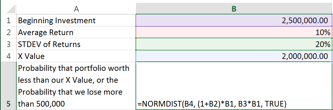
The function we’re going to use is NORMDIST, for a normal distribution. The function takes the arguments x which is the value we want the distribution for, an arithmetic mean of the distribution, standard deviation for the distribution, and cumulative which is a logical asking for TRUE is we want the cumulative distribution function and FALSE if we want the probability density function.
In our hypothetical we have been given the average return and the standard deviation, as well as the cutoff value (our “x” is just the beginning portfolio value minus our VaR). We want to return a cumulative distribution function.
Intuitively one might first try to enter =NORMDIST(2000000, .1, .2, TRUE)
After all, that uses the average, the standard deviation and the 500,000 value, right? If you try this for yourself, you’ll get a value of one – does it seem likely that there is a 100% probability of losing more than 500,000?
The problem is that the NORMDIST function wants us to use values that correspond to our “X”, not percentage returns. But its simple to convert those percentages into dollar values. 20% STDEV means that the standard deviation of our account over the course of one day (the timeframe we’re using in our hypothetical) is .2*2,500,000. Likewise, our average for the distribution is .1*2,500,000.
And the result of that function:
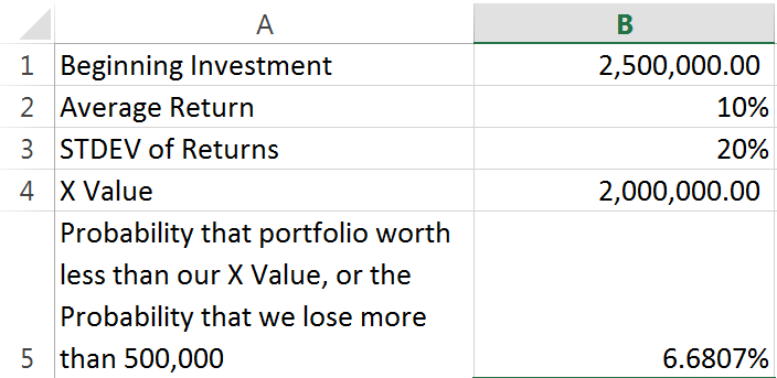
There you have it, using NORMDIST and assuming our portfolio returns correspond to a normal distribution (a common assumption though not always a suitable one), we can predict that there’s a 6.68% chance that we will lose more than 500,000 in a day. In the parlance of VaR, we would say that the portfolio has “a one day 6.68% VaR of $500,000”.
VaR is a much studied and debated concept in finance. There are many alternative calculations that aim to adjust or improve on the basic premise, some much more complicated. VaR Part II will get into slightly more complex takes on risk analysis and VaR in particular.