The two most common measures applied to proposed projects (for everything from expansion to replacing old equipment) are net present value and internal rate of return, or NPV and IRR respectively. If you don’t have a basic understanding of present value and net present value, you can get a full primer here.
A brief recap of NPV:
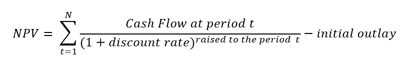
NPV is given by the equation:
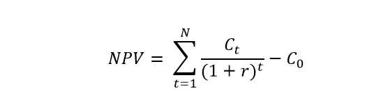
Simply put, the net present value of a project (set of incremental cash flows) is the present value of all the cash flows, less the initial outlay.
If the present value of the cash flows is greater than the outlay, then the project should be taken all else being equal. In other words, positive NPV projects get greenlit and negative NPV projects get tanked or retooled.
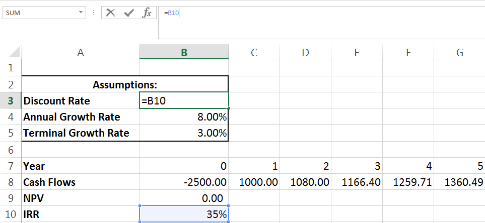
Let’s look at some hypothetical cash flows and assumptions:
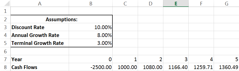
We will be discounting these cash flows using the 10% value. As you can see, cash flows begin at year 1 with a value of 1000, and then grow by 8% every year.

The excel equation used to find NPV in excel is “=NPV(discount rate, cash flow series)”. Again, you can see another basic example of NPV here.
So we’ve done this work – now what? The value we returned for NPV was positive so this project meets our requirements and, all else equal, we should recommend it. Especially given the proportion of NPV to initial outlay, its very NPV positive. To get a better feel for that, lets examine a second decision making criteria, IRR.
IRR:
IRR is the discount rate at which NPV becomes zero. If an investment has an IRR that is greater than its cost of capital (discount rate), it should be greenlit.
Let’s try to find the IRR for the cash flows we used earlier:
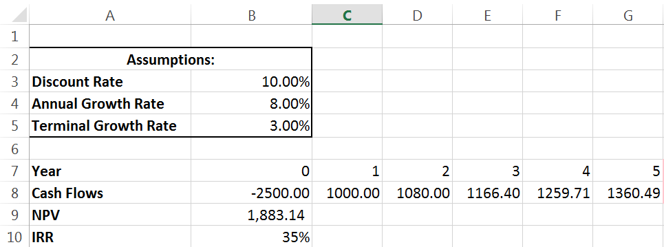
35% is a decently high IRR. This means that for this project to fall to NPV neutral (a value of zero) we would need a discount rate (cost of our capital) of 35%. We can check by setting our discount rate equal to our IRR:
As expected, when we set the discount rate equal to the IRR, the NPV in cell B9 falls to exactly zero.
One last thing about IRR and NPV is that I recommend calculating both even if only one is preferred by your organization. The reason for this is simple – you can use one to check the other. Everyone makes mistakes and typos here and there – but in the field of finance, especially regarding the decision to make an investment or not, simple typos can cost enormous sums. Whenever you have an opportunity to do a simple prodecure (like briefly setting your discount rate equal to your IRR) to check that your model is functioning as expected, you should take that opportunity.
Backing up and creating copies of models as you work on them is an important habit to get into. This is a procedure where I always back up the file I’m working with before I check for errors – IRR and NPV will often generate circular references in more complex spreadsheets. You risk breaking the model, especially if you have any VBA woven in – but thats a topic for another day.
For now, lets look at one last aspect of NPV that will have a massive impact on some investment decisions.
Terminal Values
Some projects have a definite lifespan and you can estimate cash flows for the entirety of its life. Many projects and assets, however, might not have a known end date. Take a company, for example.
If we take the NPV of the cash flows to a firm, we can come up with a value for the firm. This is obviously a useful, but how many companies do you know that advertise when they will close shop or go bankrupt? It’s uncommon. Instead, most companies are valued as “a going concern” – meaning we expect them to operate indefinitely. To solve this problem, we use a terminal value in addition to the last cash flow in our forecast period.
See the addition to the equation for NPV when we assume a going concern:
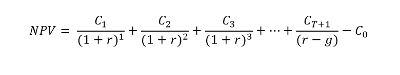
Let’s break that down a little bit:

So we add up all of the cash flows as usual, until we get to the last period (in our example, year five). If we assumed our example project would produce cash flows indefinitely, we would need to calculate a terminal value to represent its infinite future cash flows. To do this we first project out a sixth year cash flow (Cash flow in terminal period, T, + 1) which is known as our terminal cash flow. We divide that figure by our discount rate minus our growth rate. If we assume no growth in cash flows, we just divide by the discount rate – we don’t use any exponents. When we have a positive growth rate included, it makes the denominator smaller – this makes our terminal value larger. If we have a negative growth rate, then we take the discount rate and we subtract the negative growth rate from it (subtracting a negative means adding), this makes our denominator larger and decreases the terminal value.
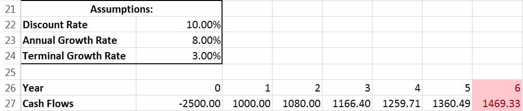
We’ll go step by step. First, we project out a year six – cash flows still growing at our annual growth rate.
To keep things clear, I’m adding a row for calculating our terminal value. A note here, we assume terminal cash flows occur in the last year of the model. Year five, NOT year six is the last year in this model. In a ten year model, we would project a year eleven only for the purpose of finding a terminal cash flow – which we would add to the existing cash flow of year 10. The idea here is that were we to sell our investment at the end of year five it would be worth the terminal value (because we’re assuming it pays cash flows in perpetuity and we have valued it as such).
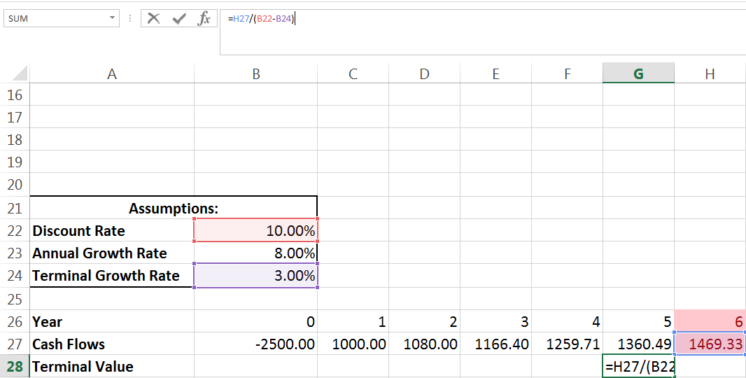
Above, we took the cash flow from year six and divided it by our discount rate (10%) minus our terminal growth rate (3%). Now we have our terminal value, we need to add the TV and the cash flow in year five together, and then calculate NPV for all of those cash flows:
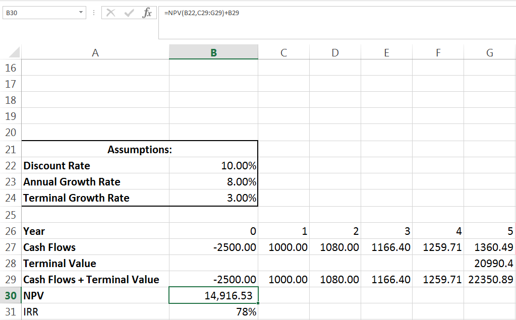
Notice a couple of things, first NPV isn’t run on cash flows alone, its run on cash flows + terminal value. Since there’s only one terminal value, the cash flows only change in one year. Also notice there is no year six! We have an initial outlay and five years of cash flows. If you compare our NPV and IRR with a terminal value to our NPV and IRR without a terminal value you can see that the project is much more valuable now. This makes sense, after all we now receive cash flows in perpetuity rather than just for five years.
A final consideration is that of terminal growth rates and their huge impact. High terminal growth rates (3% is pretty high) can inflate the value of a project massively – take a look at how much bigger the TV alone is than all the other cash flows. For this reason its important to forecast terminal growth rates carefully.
These have all been very simple examples, but they illustrate two common investment criteria.