In parallel to our ongoing series introducing different Monte Carlo techniques I thought it would be fun to incorporate more case studies and applications. Today we’re going to use a fairly basic Monte Carlo simulation to try to forecast the stock price of a small cap bank – Opus Bank, or as I’m going to refer to it, OPB. I admit that this firm is a special interest of mine, as I had the privilege of preparing an equity research report with several other excellent student analyst during my undergraduate studies. Because of that, I’m always interested to see what’s going on with the firm and its price. I’m curious – was our price target accurate?
A Quick Review
Let’s run over a few key concepts that will be key to understanding the model we’re about to put together.
First and arguably most importantly is the assumption that stock prices follow a lognormal distribution (and therefore stock returns are normally distributed.
Secondly, remember that a Monte Carlo simulation requires a set of input parameters (typically mean and standard deviation) to use for generation of random or pseudo random numbers within the model.
The Excel Method
Technically speaking all of the methods will use Excel for this series, but first we’re going to start with native Excel functions alone and zero VBA. Our first step is to retrieve the stock returns for our chosen ticker/company, using the chosen time frame and interval. In this case we’re going to look at Opus Bank, ticker OPB. We’ll use daily returns and we’ll be utilizing the entire history of its returns (it IPOed in 2014).
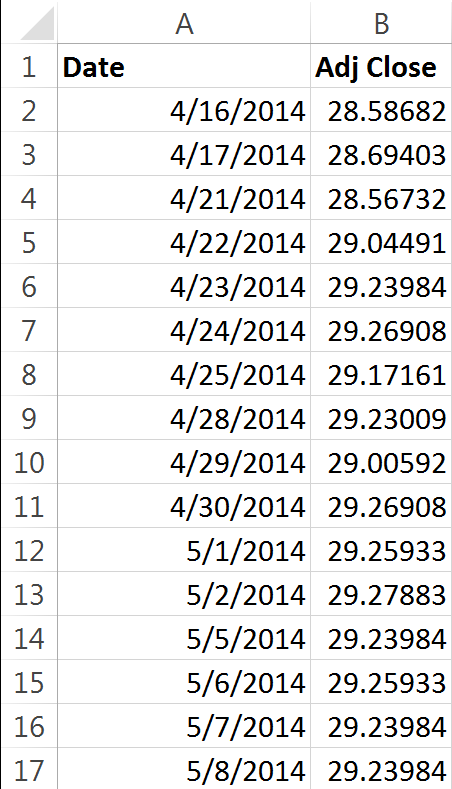
There are numerous methods to automatically retrieve stock data from various online sources but today I just went to Yahoo! Finance and manually downloaded the required data. I then edited the list Yahoo! spits out so that I was left only with a column for date and a column for adjusted return, see the set up below:
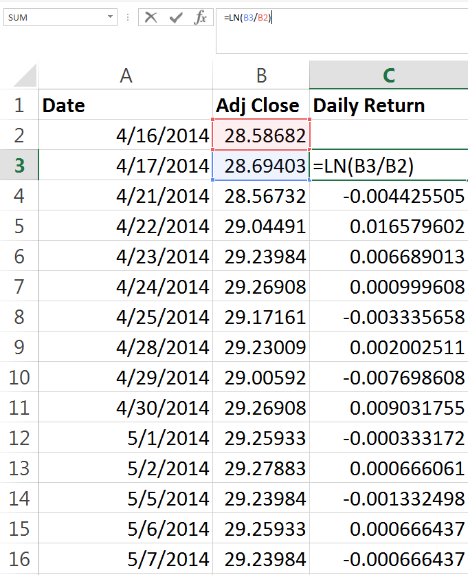
Our second step is to figure out what a typical return is for the stock, and what the risk (standard deviation) associated with a typical return is. We’ll use the LN function to determine the daily return, see below:
With this figure calculated for all of our observations, we can gather some summary statistics. Most importantly, we need the mean daily return, and the daily standard deviation. At this point we’ll also address the need to adjust the formula we’re going to be using to reflect our chosen interval. Stock returns can be measured and forecast based on minute to minute, day to day, month to month, or year to year intervals. Really, you can pick any interval you desire. Daily, weekly and monthly are the most popular intervals.
To effectively annualize, we simply divide one by the number of periods in a year. If our chosen time period is monthly for example, then we would need to use 1/12 to find our monthly return. We’ve chosen daily returns, which can sometimes confuse. A common mistake is to utilize 365 days in order to adjust returns to or from an annual basis. However, using 365 days would mean that there are 365 observations in a year. Remember that an observation in this example is a stock price – stocks do not trade on weekends and holidays. To accurately adjust our returns, we will use the figure of 252 trading days per year. Not every year has 252 trading days – but this is close to the average number of trading days per year and is a commonly accepted figure. I’ve also seen 250 and 251 used. You can see our little summary below:
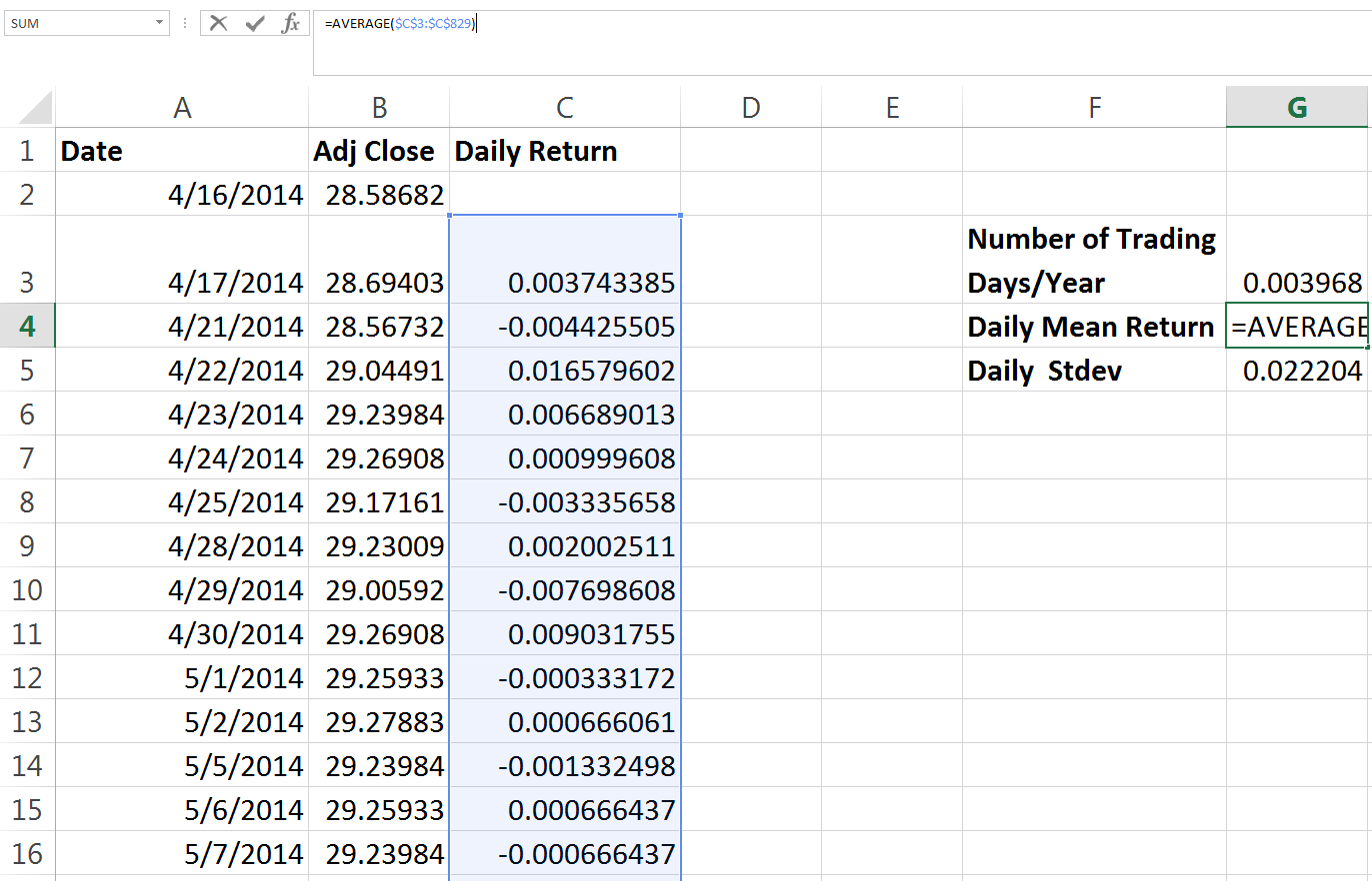
The standard deviation function is simply called on the same range as the average function is, and the number of trading days/year (somewhat confusingly named, I apologize) cell contains the formula “=1/252”.
Now we can get into our real forecast. First, we want to take a number of days from zero (to reflect todays price) all the way down to 252 (we want to forecast the price one year out). With that column established, next to it we will enter an equation which may at first seem a little confusing and intimidating. For more detailed discussion and explanation of the relevant equations, you can see this discussion of lognormal stock price distributions and conversion from normal to lognormal.
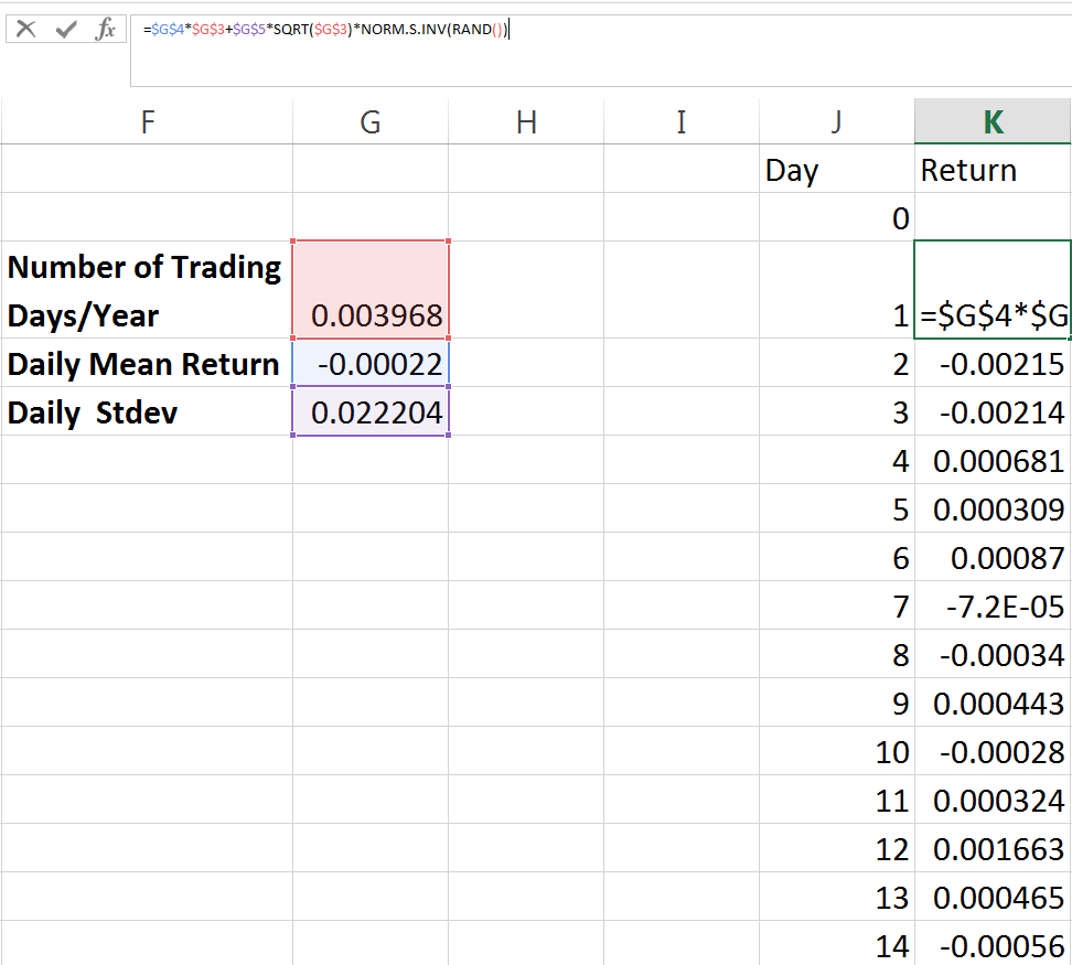
With this equation, we’re utilizing the three inputs we defined. We have the time interval, the mean daily return and the standard deviation of daily returns as well as our pseudo-random number generation.
This gives us our daily expected returns, and we can use it to calculate the expected return a year from now. Before we do that however, what if we’d also like to easily see the expected price on a given day between today and one year from now? We can use the following equation to adjust the returns into the stock price. Notice that it begins by referencing the previous days stock close and then increases or decreases it by the return we’ve calculated.
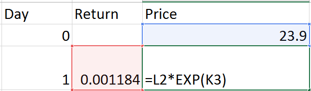
The formula being used is just the previous days stock price multiplied by EXP(current days return). This should make some sense intuitively, as we’re just using the current days return in our e function and multiplying that by the previous days close. With that work done we can now go find the closing price in one year and the expected return over the entire year.
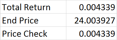
We can also quickly check our math to make sure that our closing price in one year and our expected return over one year line up. We can do this by finding the return between our day zero stock price and our forecast stock price one year from now using LN – the number we get should exactly match the cumulative return that we randomly generated since our closing price is based on that information. If the two don’t match then we know we have an issue somewhere, probably with cell referencing (perhaps we forgot to make a reference absolute) and we need to check our work closely. As you can see above, the two match up so we know we’re using consistent formulas. Granted, we may still have made a mistake – but if we did its been made consistently and I always feel a little better after running any kind of double check on my own work.
This outlines the basic process but represents just one simulation – Monte Carlos use many thousands. Next we’re going to manually copy the results of our forecast price column into several nearby columns. Since we’re using RND() in our function, and its volatile, after each time we paste the values from that column into a new one, all 252 prices will be recalculated. This effectively means we can copy the results of one simulation, and immediately excel will have “run” another one for us to copy. This is a boring and labor intensive process to even get a small sample of simulations but it further illustrates a process we’ll automate with VBA:
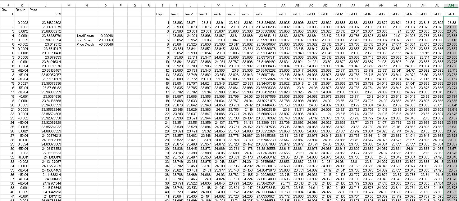
The shot above shows immediately after using excels paste values command to copy the “Price” (Column L) simulations into “Trial 20” (Column AM). As you can see, the pasted prices in Trial 20 are now different than the prices that Excel is calculating using our equation. This took just a few seconds, but 20 is a tremendously small sample size. Imagine trying to get 1000 samples for a project this way!
Even though we have a small number of simulations, I’m a firm believer in practicing all aspects of analysis in Excel. This includes generating a visualization of the model and its output, so lets throw in a quick chart:
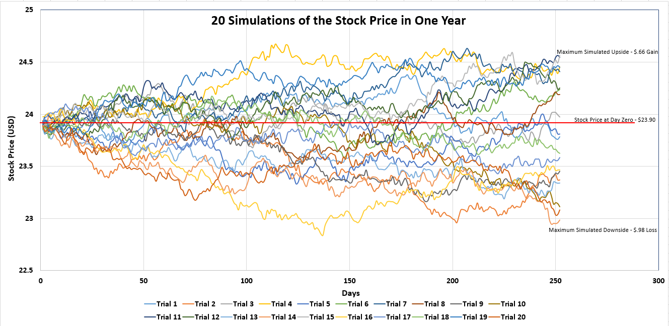
Building the chart took a little longer than copying the data 20 times, but which one provides more information to the end user? If you had to sit through me presenting the results of these 20 simulations to you, would you prefer I have this chart or the table with all 20 trials above it?
The results aren’t especially meaningful in my opinion, due to our small number of simulations. However, you can see that generally they conform to the results we would expect given the average daily return for OPB was a small negative number. We have more simulated outcomes that result in a one year close below its close today and the largest simulated downside is much larger than the largest simulated upside.
As we continue to explore using Monte Carlo to model future stock returns, we’ll examine the impact of changing the interval from daily to weekly to monthly. We’re also going to examine automating these processes with VBA so that we can run many more simulations. Then, we’ll take a look at the best ways to visualize many thousands of simulations – without attempting to graph each simulated outcome individually. Finally, we’ll build a model that takes into account more interesting parameters than just mean and standard deviation of historical returns.
For more practice using Monte Carlo, you can also take a look at some coverage of their application for risk analysis.
Here’s Part II.