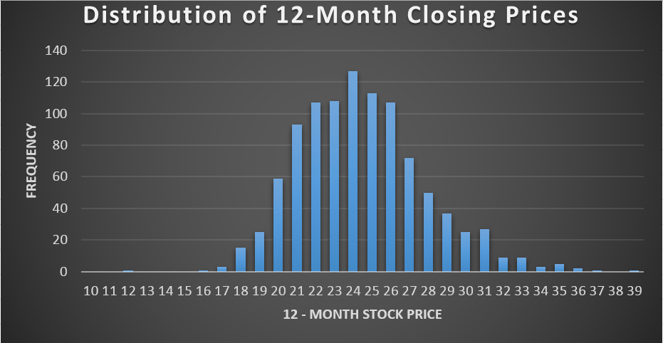
Following up on Part I, we’re going to kill two birds with one stone and learn both how to simulate one years stock performance based on historical returns and examine OPBs monthly returns instead of its daily returns. The end goal is for us to create a set of simulations that can help us learn more about the probable performance of the stock and enable us to build some powerful visualizations to communicate that information quickly and efficiently. One good example is a simple histogram:
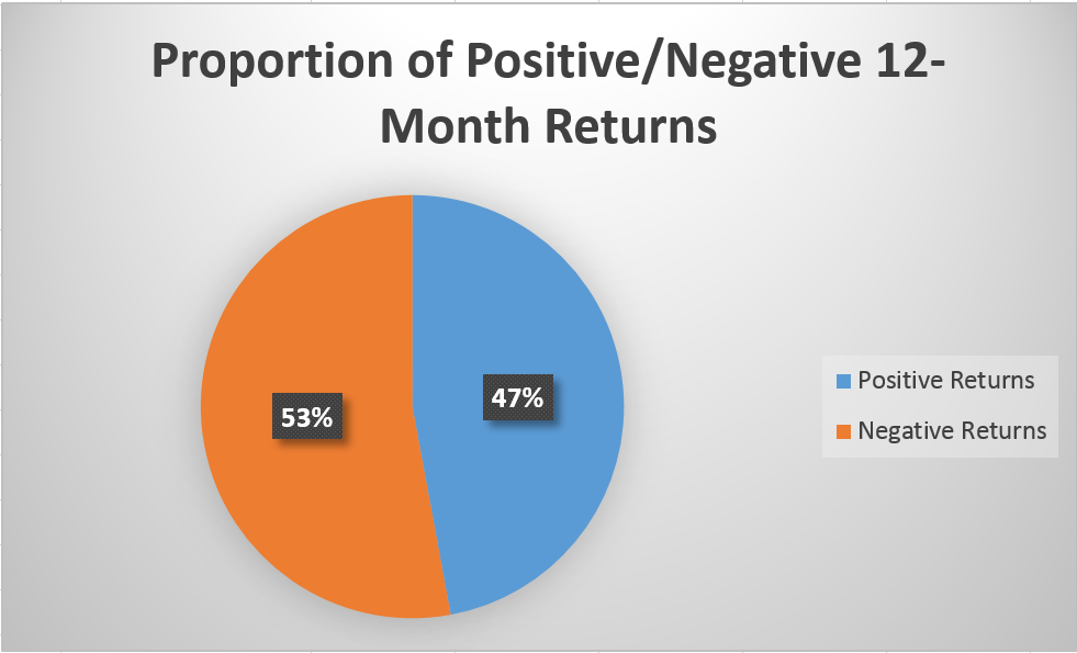
We could also easily look through all our simulations to find the percentage of closing prices above and below the most recent close – giving another easy way to picture the likely performance of an investment in OPB (based on this analysis alone):
So that’s our goal, let’s get into the VBA editor and start to work.
Data and Returns
I manually grabbed all of OPBs monthly stock returns from Yahoo! and removed everything but the date and adjusted close columns. I also deleted the last row of data, since its for an incomplete month. With the data ready to go we can start to code a little.
My actual data runs from A2:B40, with all of the adjusted monthly closes in column B running from B2:B40. This is the column we’re most interested in.
Out of habit from testing models as I build them, I first named the sheet I was working with “Data” and set it to be the active sheet when the code is run. I also defined a few variables we’ll be using. Have a look at my initial code:
Dim Historical() As Variant
Dim Returns() As Variant
Dim Deviations As Variant
Dim MeanReturns As Variant
Dim Simulations As Long
Dim Period As Double
Dim MonthlySim As Double
Dim LastPrice As Double
Workbooks(“StocksWithVBA”).Sheets(“Data”).Activate
Historical = Range(“B2:B40”)
LastPrice = Range(“B40”)
ReDim Returns(1 To UBound(Historical) – 1)
For i = 1 To UBound(Historical) – 1
Returns(i) = Log(Historical((i + 1), 1) / Historical(i, 1))
Sheets(“Data”).Cells(i + 2, 5).Value = Returns(i)
Next i
So first we define data types for a long list of variables. You can ignore most of those, we’ll explain each one as its used. The first real action we take is to activate the sheet containing our stock data, then we set a variable named “Historical” as the array from B2:B40, which is all of our returns. We also create “LastPrice”, which is equal to the value in B40 – our last monthly return and last price. We’ll use that variable later on.
Following that we make an adjustment to our previous dimension for the variable “Returns”:
ReDim Returns(1 To UBound(Historical) – 1)
In a nutshell, this line of code says that Returns will be match up with the length (UBound, or upperbound) of our Historical variable, less one. We make this adjustment to reflect the fact that we will have one less number of “returns” than our number of historical monthly prices. As arrays of data, the two will be of unequal length – you can check out Part I to verify this. The very top cell of the row we used to calculate our daily returns was empty because there’s nothing to compare our earliest observation to in order to get a return.
With that housekeeping out of the way, we run our first loop:
For i = 1 To UBound(Historical) – 1
Returns(i) = Log(Historical((i + 1), 1) / Historical(i, 1))
Sheets(“Data”).Cells(i + 2, 5).Value = Returns(i)
Next i
If you break this down, it should look familiar to the same step we did for the Excel only method in Part I. We just compare each months stock price to the previous months stock price, taking the natural log of the newer observation divided by the older observation. We write the result of that calculation into the corresponding adjacent cell in column 5 (Column E), and then we repeat the loop. The loop is continued, calculating the month over month log return until we reach a number of loops equal to the upper bound of our historical array, less one.
With that finished, we can collect our averages and standard deviation:
MeanReturns = Application.WorksheetFunction.Average(Returns)
Range(“E1”).Value = MeanReturns
Deviations = Application.WorksheetFunction.StDev(Returns)
Range(“F1”).Value = Deviations
Writing the average and standard deviation into actual cells is entirely optional. The main reason I do this for a lot of variables and intermediate calculations is so I can run the calculation by hand to test that the VBA is working correctly. I think it’s worth taking the time to confirm the results of your VBA the first time you use it – if possible. After you’ve tested each component or segment, you can comment out the offending bits of code and sleep easy.
The Simulations
With our historical returns, averages and standard deviation gathered we can now begin to actually code the model. Let’s handle some preliminary definitions:
Period = 1 / 12
Simulations = 1000
n = Simulations
We’re using monthly returns, so we need to remember to incorporate that by dividing 1/12 and storing the result. We could of course also just use 1/12 in the actual formula, but should we want to change this to a daily model we’d have to manually edit each piece of code where we use this information. This way, we would only have to make one change.
I’m arbitrarily using a thousand simulations. This is on the low end for a Monte Carlo but will still take a few minutes for most computers to complete. The first few times I ran the full code I ran it with 100 simulations so that bug checking was faster.
I’ve also defined n as simulations, so n will also equal 1000. This is an entirely optional step as well. My last step was to insert a new sheet (manually) into the workbook and label it “Output”. Here’s our loops:
For k = 1 To n
For i = 1 To 12
Sheets(“Output”).Cells(2 + k, 1).Value = k
Sheets(“Output”).Cells(2 + k, 2).Value = LastPrice
Sheets(“Output”).Cells(2 + k, 2 + i).Value = Sheets(“Output”).Cells(2 + k, 1 + i).Value _
* Exp(MeanReturns * Period + Deviations * Sqr(Period) * _
Application.WorksheetFunction.Norm_S_Inv(Rnd))
Next i
Next k
Workbooks(“StocksWithVBA”).Sheets(“Output”).Activate
First we’re saying that we’re going to loop through from 1 to our number of simulations (“n”, in this case a thousand). The thing we’re going to do 1000 times is another loop. This loop is going to get run 12 times, and will end up writing output into a row of cells each time its run.
First we’re writing the value of “k” into the first column, starting with the third row (2+ k, and k begins with 1). Since we said that k would loop from 1 to n (which is 1000), we’ll end up with values of 1, 2, 3, 4, etc all the way down to 1000.
The next output is calling up that “LastPrice” variable we created, and it gets written in the second column, right next to its simulation number, for every single row we run our loops on.
The main portion of our loop is a little gnarly, but it could help to go back to Part I. Remember how we had one long equation for finding our randomized returns based on the mean and standard deviation? And then with that we could take the previous periods stock price and multiply it by e raised to the power of our randomized stock return for the current period? That gave us our new stock price.
This code is doing all of that at once. To find the previous months stock price in each simulation (remember each row is a different simulation) the code will take the value in the preceding month (column), and multiply that by e raised to our formula.
You can see how this is working by comparing the cell we’re writing to during each iteration of each loop, to the cell its including in its calculation:
Sheets(“Output”).Cells(2 + k, 2 + i).Value = Sheets(“Output”).Cells(2 + k, 1 + i).Value
I’ve underlined the critical reference. In blue, we have the row that our VBA is working in. Notice its the same row within this loop – this is good, we want to stay within the same simulated set of monthly prices.
In red, we have the column references. Those are different. The cell we’re writing to is 2 + i, while the cell we’re referencing is 1+i, a cell “behind” us, aka the previous month. This is why we took the time to write in our last known historical closing price, “LastPrice” into every single cell of the second column – now the first month we simulate in each year has a price to refer to. Also its nice and uniform this way.
The code works by looping through a row of cells, starting from the third columm (2 + i, and remember that i begins at 1) and completing our calculation 12 times across that row (because we said “For i = 1 to 12″). The row is determined based on k, so we’re going to write in our stock prices for all 12 months in a row, and then another row, and then another row, filling down the worksheet until we reach our set number of simulations.
I threw in a command to make sure we activate our output sheet at the end to make testing the code a little easier – its totally optional and unnecessary once we’re live. Take a look at the first few simulations created entirely through our code below:
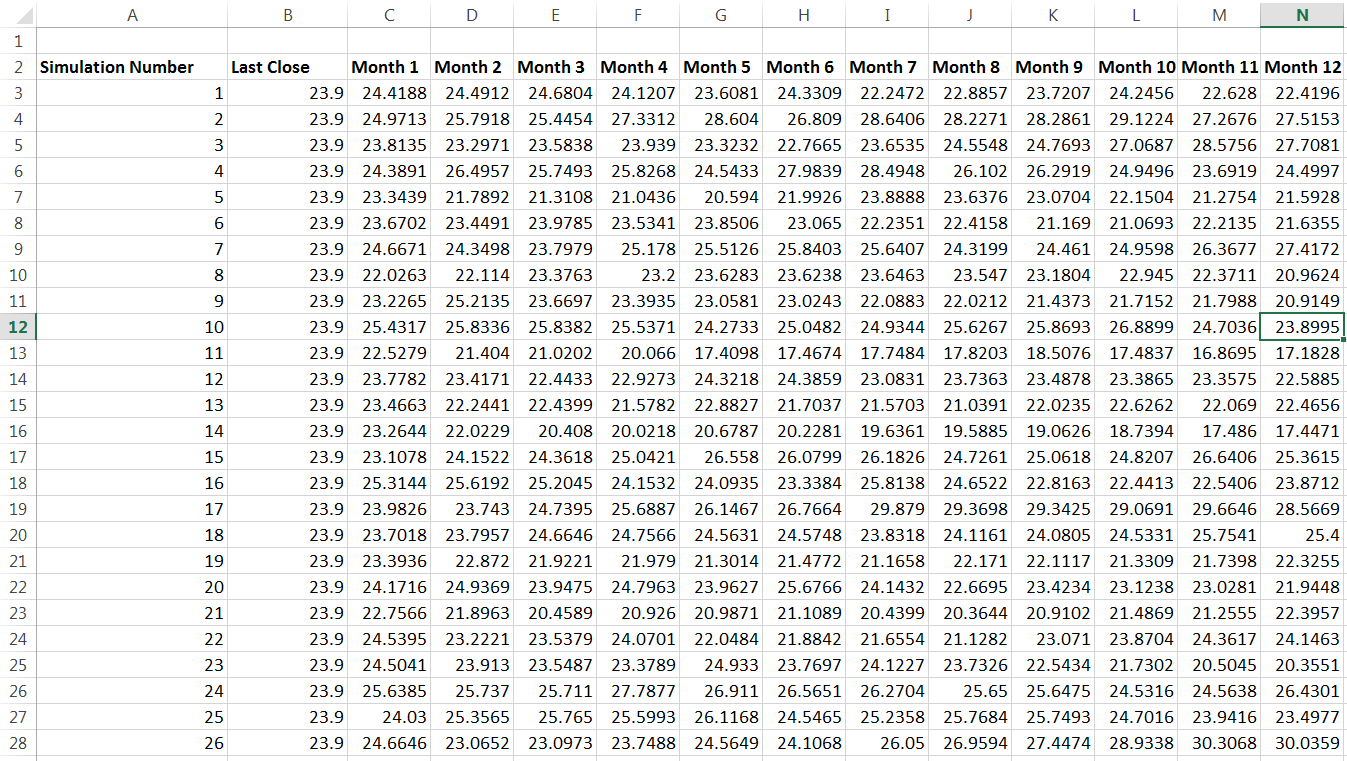
The labels at the top I wrote in manually, the rest was entirely done through VBA. This fills down a thousand rows. While vaguely interesting to look at, it’s a huge pain to try to get any truly useful information out of the table alone. You can compare this to the pie chart and the histogram at the top of the post and decide which one tells other people more about your analysis. Remember, if the consumer of your analysis (your boss, a professor, whomever) cant understand the output then all the work you’ve done hasn’t created any value.
We wont go into histogram or pie chart creation. The pie chart is pretty simple to figure out. Here’s a hint, I used COUNTIF. The histogram and creating bins has been discussed a couple times already here at 440.