What is Covariance?
Covariance is simply the variance between the observations of two random variables. It should be clear both from its name and the brief description I’ve provided that covariance and variance are quite similar. Recall that variance measures the (squared) difference between what we expect from a variable (its mean) and what actually happened. Covariance uses similar math, but instead of comparing observations of variable, X, with it’s own mean (which is what variance does) we can use covariance to compare it with the observations of another variable, Y.
Why Should You Care?
Consider a portfolio built out of two stocks which move together. In this case, our risk is substantial because both stocks will decline simultaneously. If we select stocks that have a low covariance, or negative covariance (indicating an inverse relationship) we can lower the risk of our entire portfolio experiencing decline at the same time. Across a portfolio that consists of many stocks we can use this process for the entire portfolio, optimizing it so that we maximize returns at a certain desired risk level or minimize risk at a desired level of return. Utilizing covariance is just one part of creating optimized portfolio’s, and there are methods that do not utilize covariance at all – but its a common and respected methodology and thus worth discussing and learning.
The Equation and Some Properties to Remember
- Covariance is going to be higher among datasets that you can fit a line of positive slope to.
- Covariance decreases as the slope of the line of best fit decreases/becomes negative.
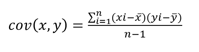
Let’s break the equation down.
The covariance of two variables (let’s assume they’re stock returns) X and Y, is given by the sum of: each observation of X (represented by Xi in the equation) less the sample mean of X, times the corresponding observation of Y (Yi in the equation) less the sample mean of Y. Once you’ve done that calculation and summed the results, you divide by the sample size, n, less one.
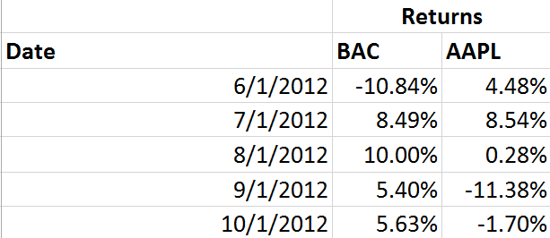
We’ll go through an example using five months of return data for BAC and AAPL, from June 2012-October 2012. The monthly return for each stock is shown below:
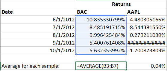
Taking that data, we should first find the average return for both AAPL and BAC:
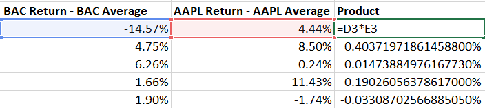
With that done, we’ll keep going step by step and subtract that average from each observed return for both AAPL and BAC, respectively:
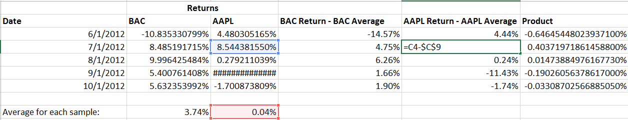
Then, we multiple each of those results together.
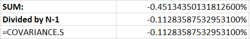
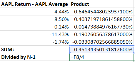
Finally, by summing the result we’ve completed the numerator of our equation.
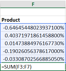
Now we just divide by our sample size (5) less one.
To check our work, let’s use excels built in COVARIANCE.S function (the .S signifies its for a sample of data):
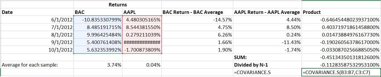
As you can see, it checks out. Breaking it down step by step is useful for learning covariance but is obviously extremely time consuming compared to a built in solution like COVARIANCE.S.