For a quick overview of Monte Carlo simulations, I recommend you check out Part I.
Example:
Suppose we work for a small clothing manufacturing company in the midst of a lawsuit. Apparently, our firm allegedly dumped a little bit of excess blue dye into a nearby lake and turned a hundred nearby campers blue. Predictably, government regulators have levied a fine that is due in one years time and the campers have filed a joint civil suit as being dyed blue was not to their liking.
The company failed to reach a settlement after offering each plaintiff $1000 and is going to court in a case that will take a year. It’s possible the company will win, and have to pay out no money. It’s also possible that the firm will have to pay the maximum penalty allowed by law – $3,000 per plaintiff. Obviously there’s quite a bit of variability between $0 (we win) and $300,000 (we lose and pay the maximum penalty to each of the one hundred plaintiffs).
This makes planning for the future difficult – our management doesn’t know how much money they should prepare to pay in a year. If they set aside the maximum and it turns out we win, they may have lost the opportunity to invest that money in projects that could grow the business or increase its margins. If they set aside too little, they may have to scramble to come up with extra cash when the court case is decided – that could mean taking a loan or being forced to sell some current assets.
In this case, our company had been planning a major capital investment and senior management needs to know how likely it is that the company will need to pay out more than $200,000. Any more than that and the firm needs to put its investment plans on hold.
This is where the vaunted Monte Carlo comes to the rescue – we can use our simulation to give good guidance on the subject to management.
To find out how much money the company will need to cover this incident in a year, we can write an equation that captures the cost per plaintiff as well as the fine already levied by the regulator (due around the same time as the case is expected to be decided):
Total cost = 15,000 + cost per plaintiff * number of plaintiffs
This should be familiar as its a linear equation (y = mx +b).
If we are feeling lazy, or are unfamiliar with Monte Carlo simulations we might do an uninspired analysis through a simple what-if data table:
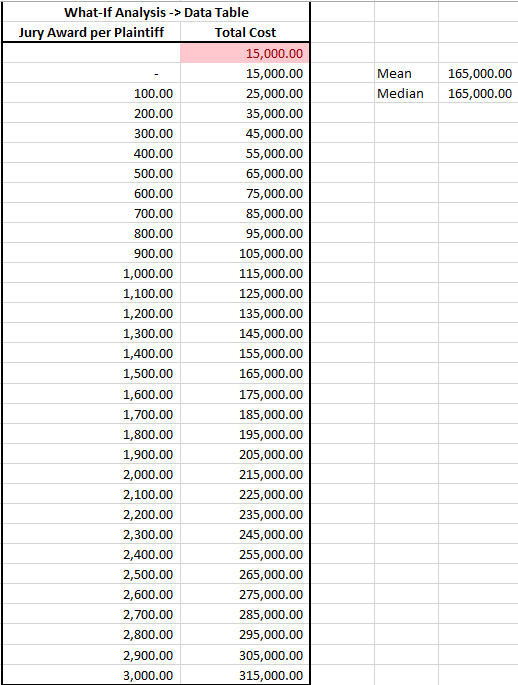
Off to the right you can see I calculated the mean and median for all our these outcomes. They’re exactly the same. So we could take this to management and tell them the most likely amount the firm will need to pay is $165,000 (this figure is $15,000 for the fine plus $1,500 per plaintiff). Realistically though, all we did is take the midpoint of all possible jury awards – we have no idea if this is a likely outcome or not.
Our management is understandably displeased and we are told to do a more thorough analysis. Remembering something about a “Monte Carlo”, we decide to throw something together.
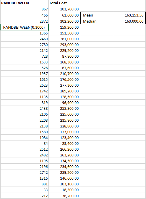
We’ll use the excel function RANDBETWEEN, which returns a random figure (uniformly distributed) between two values we enter. We type in “=RANDNUMBER(0,3000)” and drag it down a thousand cells. Then we write in our equation to the total cost next to it, giving us the total cost for reach random jury award and calculate average and median figures for the total cost. Now we can claim we used a “stochastic process with a thousand simulations” to arrive at our recommendation. Heck, we can make it more impressive. Let’s drag those formulas down to 100,000 cells. Now we used a stochastic process with “one hundred thousand simulations”. We’re good to go! Here’s the top part of our incredibly long table:
We’ll even toss in a frequency distribution for our presentation, management likes charts and graphs:
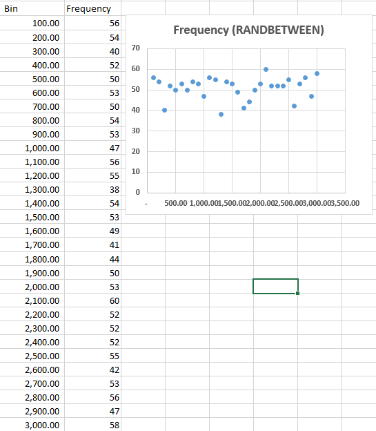
One could argue that this technically counts as a Monte Carlo simulation. I think that’s a very week argument in this case though, and if you know how RANDBETWEEN works or take a close look at our distribution you’ll be able to guess why. RANDBETWEEN selects random numbers based on uniform probability. So we’re equally as likely to get a value of 1 as we are to get a value of $2,500.
This is sort of a lynch-pin of effective use of MCs, in my opinion. You have to select the correct probabilities for your random number generation. If the input you’re running the simulations for really does tend to be uniformly distributed (say we had studied jury awards in cases similar to ours and found that they’re just as likely to award any number between the max and the min), then you need to use random numbers generated based on that distribution. If your input tends to vary in a normal distribution (common), then a uniform distribution is absolutely the wrong method to use.
Additionally, with one input being tested and no additional tweaks to the model – you can see that we get very similar mean and median values as just creating our linear data table. We haven’t added a lot of value or insight to the decision making process – yet.
Earlier I mentioned that normal distributions are common. These are distributions where you a higher probability of getting a value close to the mean than one that lies far away from the mean (distance from the mean being measure in standard deviations).
A right way to do it:
We’ve built a datatable – no good. We created our first stochastic process, fine for uniformly distributed inputs, but not quite good enough. We didn’t do any actual research to discover if juries assign awards in a uniform manner or not – we just assumed they did. The actual distribution of jury awards is a subject of study though, and we can find some interesting information about their distributions for various types of cases. Here, let us assume that we’ve discovered based on our research that for this particular type of civil lawsuit jury awards on a per-plaintiff basis tend to follow an approximately normal distribution, with an average award of $1,100 and a standard deviation of $400.
We can now use NORM.INV and RAND() along with our mean and standard deviation to create a set of simulated outcomes that can add some real value:

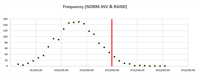
Givings us the following distribution:

With the hard work done we can also create a set of bins and frequencies for the total cost – the first bin is $15,000 (our minimum cost) and the last is $315,000 (full award plus the fine). This will give us a neat visualization that conveys a lot of information about the likelihood of our costs exceeding managements $200,000 figure – remember the key third element to a good Monte Carlo. We can add a quick vertical line to the chart to make it even easier to understand at a glance, and normally we’d want to have a more descriptive title and axis labels, but for our purposes today this will do:
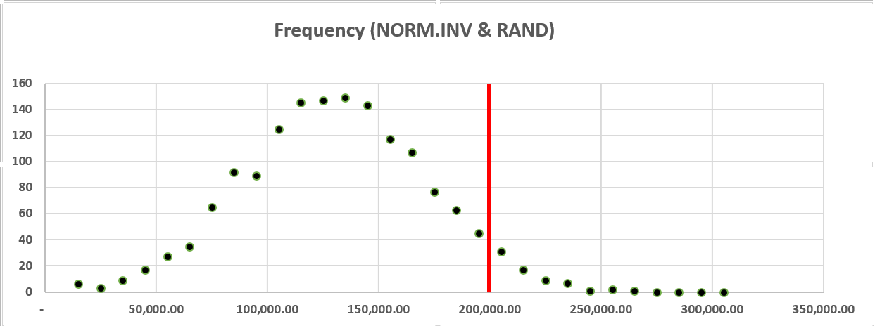
Finally we can use NORM.DIST one last time to give us the probability of getting a value that is less than or equal to $200,000. If we subtract this probability from one, we have the probability that the firm will have to pay out more than $200,000:
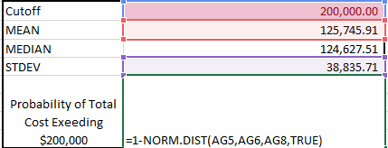
Here I’m taking the average total cost of all the simulations and the standard deviation of the total cost of all the simulations – so any time you hit F9 you’re going to get a slightly different figure for this probability. The equation used for finding the probability is”=1-NORM.DIST(Cutoff amount, mean, stdev, TRUE)”
There, that’s all a Monte Carlo simulation is. This is obviously a very simple one with a nice normal distribution and only one input variable, and no code. Additionally, most MCs will run more simulations than we did. This means that we can get a very good idea of our probable outcomes. If you increase the sample size here to say, 10,000, and hit F9 a couple times you’ll see that there’s less change in our probability of exceeding $200,000 in total costs.
A Fly in the Ointment
One thing we didn’t address is that as we generate our jury awards we don’t want any that are less than zero or more than 3000. Based on the standard deviation and mean we specified, such outcomes are unlikely – but if you do enough simulations you’ll find them (a negative jury award would be less than 3 standard deviations from the mean). Using a bit of VBA (which will get into during Part III) I applied our formula to 100,000 cells and then used COUNTIF to find those where jury awards were negative, and as we might expect given our mean and standard deviation we end up with about .3% negative jury awards – an impossibility in our scenario.
Within our random number generation it can be difficult to add additional constraints such as this without resorting to code or excessively long formulas. VBA is the ideal way to handle this type of thing, in my opinion. However, you can probably imagine that we could also solve the problem in excel either inside the formula we use for our simulations (it’s long and confusing, and won’t be appearing here) or we could modify our bins and gathering of statistics based on our simulations using COUNTIF to control for results that are out of bounds. These could be removed entirely, or counted simply as either minimum or maximum acceptable values (zero and 3000).