A Time-Value of Money
Arguably the most fundamental concept in finance is that of a “time-value of money”, where the present value of an asset or liability and its future value are not equal. Momentarily, lets set aside economics and theory for a moment and think selfishly. Generally speaking, what we mean by a time-value of money is that a dollar in your pocket today is worth more than a dollar in your pocket tomorrow. This is also true of a larger sum.
Consider the choice between receiving $100,000 today and receiving $100,000 thirty years from now. Which would you prefer to have? The majority of people would select $100,000 today. Perhaps you have credit card debt, or student loans which you would prefer to pay off now. Perhaps you’d like to purchase a house or new car and need the money for a down payment. Maybe you’d choose to invest the money today with the hope and belief that in thirty years you would have far more than $100,000.
All of those hypotheticals represent opportunities that may only exist for you today or may be more important or valuable for you today. As you can see there are opportunity costs to deferring your receipt of $100,000 by thirty years. This is why we say that there is a time-value of money. In finance we place a special emphasis on the opportunity cost of investing the money today (as opposed to costs such as buying a car or paying off loans, which vary greatly from individual to individual).
Let’s suppose that you take your $100,000 and invest it in an index fund. Let us also suppose that the stock market is expected to increase by an average of 5% every year. After thirty years, you would have $432,194.24 in your account – more than 400% above what you would have in thirty years if you deferred. Obviously, taking the money today is more valuable to you than taking the money later.
But how did we reach that figure? This brings us to some math, bear with me.
Present Value and Excel
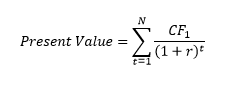
Where:
t = the time period of the cash flow
CF = the cash flow
r = the discount or interest rate
The equation above may appear intimidating at first, so lets break it down. In plain English we take each cash flow, and we divide it by (1 + r) raised to its time period, t. That calculation gives us the present value of every single cash flow provided. With the present value of each cash flow in hand, they are all represented by their value in today’s dollars and we can add all of them to get the total present value. In the example we’ve been working with, there is only one future cash flow to convert to its present value – $100,000 in thirty years. You can try the math yourself by hand, but whenever possible it’s preferable to make life easier with excel: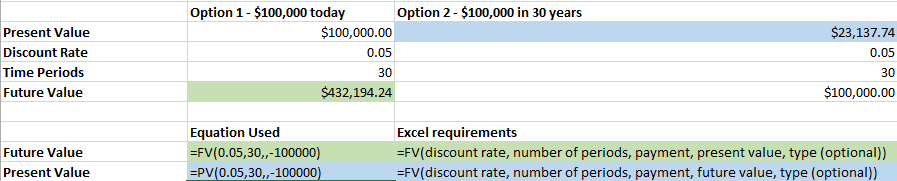
** In the examples I’m using, I’ll sometimes leave out cell references so that you can easily see what value is used in the function (seeing “.05” for interest rate instead of “B6” makes it easier to understand new excel functions, in my opinion). However, financial models should be built flexibly whenever possible – this means writing in values instead of using a relative or absolute reference should be a rare occurrence. **
The two key equations used here are PV and FV, which stand for present value and future value, respectively. Each input in the function is called an argument, PV and FV both have five arguments. Each argument, or input is separated by a comma. Notice that in this example, there are no payments – just a lump sum now or a lump sum in thirty years. Because of this, where excel usually asks for the payment, we don’t enter a value and simply place another comma. This tells excel to ignore the payment.
We also don’t specify a value for the type. By default excel assumes that payments are made at the end of the period, the type argument can be used to specify that payments are made at the beginning of the period instead, such as with an annuity due as opposed to ordinary annuities.
Now that we’ve illustrated both the concept of a time-value of money and gotten our hands a little dirty with excel, let’s take a look at one more example – this time with payments thrown in as well. Suppose we have the opportunity to purchase a bond that will pay us $1000 at the end of every year for five years, and will pay us its face value of $100,000 at the end of year five as well. The discount rate is still 5%. How much should we be willing to pay for this investment? By using the excel PV function, we can find out.
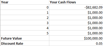
In year 0, today, I used the PV function to calculate how much you would have to pay to receive that bond – in this case it will cost you just under $83 thousand. This might seem like a good deal until you remember the time-value of money and that 5% discount rate are automatically taking into account the opportunity cost associated with losing that money today. This is not a good or bad price – all else equal it is a fair price. You can confirm this for yourself by utilizing the FV function in excel.
The PV and FV functions are useful for all sorts of investment decisions, but they are limited. Notice how the payments over the course of the investment have been fixed – they’re all the same amount. What about investments that will pay different cash flows?
NPV and Excel
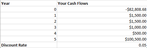
Lets make some small modifications to our previous example. Let’s say that our investment now will pay us $1500 for the first two years, $1000 for the third year, and then $500 for years four and five. The discount rate is still 5% and the face value we’ll receive at the end of year five is still $100,000. Given payments that are no longer fixed, we cannot use PV to find the value of the investment today. Instead, we can use an NPV function. See below:
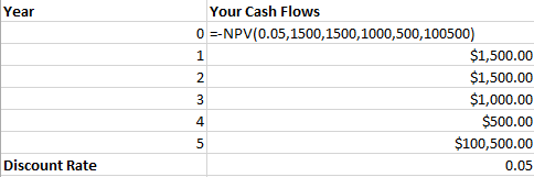
The first argument for NPV is the discount rate, just like the PV and FV functions. After that however, you can enter each cash flow (separated by commas) individually – even if they’re of different amounts. I put a negative sign ahead of the function because in year zero this investment will be costing you money, but it doesn’t change any of the figures.
As you can see, the present value of this investment is slightly higher than that of our previous example. If we look at the changes made to the cash flows, we can see why. By changing the first two payments to $1500, and the last two to $500 while keeping the payment in year three flat at $1000, we are receiving more money early and we can reinvest that money quicker at the 5% discount rate. This adds value compared to the payments being level at $1000 over five years.
NPV – Net Present Value?
Notice that I never told you what NPV stands for. That was intentional. NPV is a misnamed formula – the letters stand for “net present value” – but thats not what the function does. As we just saw, filling all of the arguments in the function (discount rate and then cash flows) actually returns the present value. There’s nothing net about it. If we want to find the net present value of something, we simply take the present value of the investment and we subtract what we paid for that investment. If we paid more than the present value, the investment is said to be net present value, or NPV, negative. This is almost always undesirable. What we want is positive NPV, where we pay less today for an investment than it is actually worth in today’s dollars.
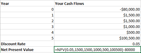
Let’s take a look at the previous example – but this time let us say that you have been offered the investment for a price of $80,000. Intuitively, since we have changed none of the inputs you should be able to guess that this will result in an NPV positive investment for us.
To find a true net present value using NPV, we calculate use the NPV function as normal and then outside of the parenthesis we subtract the cost of the investment. The cost of the investment in year zero should absolutely not be included within the parenthesis, or used as the first cash flow. Remember, each cash flow is being discounted in this function! The first cash flow entered is computed by excel to be a cash flow at time period = 1, and not time period = 0. This is a common mistake in financial models.
How much money did our investment net us? Try it out and let me know!